Next: Bayesian Adaptive Kernel Estimates Up: A Bayesian Kernel Density Previous: A Bayesian Model
As a first example, consider an MCMC analysis of the model and data described in Naylor and Smith (1988). This concerns inference about five dates forming boundaries between differing, distinct, and abutting periods of pottery production. The data consist of radiocarbon date determinations associated with pottery fragments identified as belonging to one of four periods of pottery production.
Their analysis obtains a posterior density
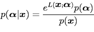 |
(10) |
where
![]() is a vector of dates before present2 (BP)
is a vector of dates before present2 (BP)
![]() , having prior
, having prior
| (11) | |||
| (12) |
![]() is the normalizing constant.
is the normalizing constant.
![]() is the Log-Likelihood
is the Log-Likelihood
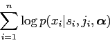 |
(13) |
where
 |
(14) | ||
 |
(15) | ||
| (16) | |||
 |
(17) | ||
![$\displaystyle b_i^{-1}\left\{\Phi\left[\frac{a_i+b_id_i(j)-x}{s}\right]
-\Phi\left[\frac{a_i+b_id_{i-1}(j)-x}{s}\right]\right\}$](img75.png) |
(18) |
![]() being the standard Normal distribution function and
being the standard Normal distribution function and
![]() are values
expressing a piecewise linear radiocarbon calibration curve
(Clark, 1979).
are values
expressing a piecewise linear radiocarbon calibration curve
(Clark, 1979).
| (19) | |||
| (20) |
where here ![]() is the actual date of manufacture.
is the actual date of manufacture.
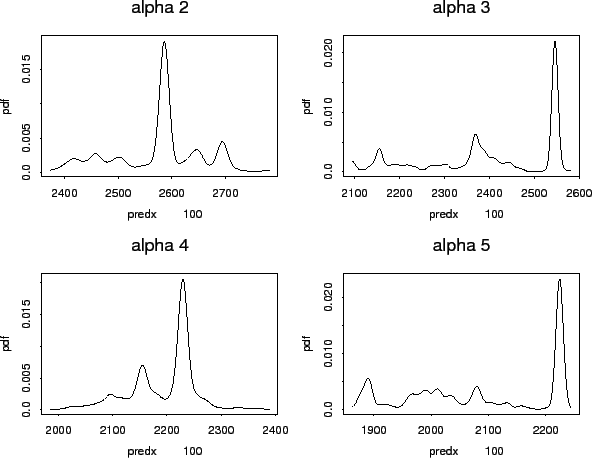
The analysis presented here, using MCMC, incorporates into the likelihood a calibration curve, defined by Clark (1979) in piecewise linear segments, relating radiocarbon date to calendar date. This curve includes inversion (i.e. it is not monotonically increasing), which renders its use difficult. Figure 1 shows univariate posterior densities estimated using BKDE for four of the five boundary dates.
Taking
![]() (ensuring that the estimate of
(ensuring that the estimate of ![]() at
any point is positive) to have prior
at
any point is positive) to have prior ![]() , represents a loosely
held belief (
, represents a loosely
held belief (![]() ) that the density is smooth (
) that the density is smooth (![]() ), corresponding to
), corresponding to ![]() . That is
. That is ![]() in the range
in the range
![]() to
to ![]() being considered probable a priori.
being considered probable a priori.
These densities are seen to be considerably less smooth than the corresponding results of Naylor and Smith (1988) who used an older, but smoother, calibration curve. There is some evidence that the likelihood is not smooth and other authors have found that there are considerable problems for maximum likelihood analyses (Clark, 1979; Cunliffe, 1984).
The analysis returns as many points as required. In this example
![]() points were generated and then reduced to 500 by extracting
every 20th result
3.
Taking
points were generated and then reduced to 500 by extracting
every 20th result
3.
Taking ![]() , a uni-dimensional likelihood is constructed with one previous
sample.
, a uni-dimensional likelihood is constructed with one previous
sample.
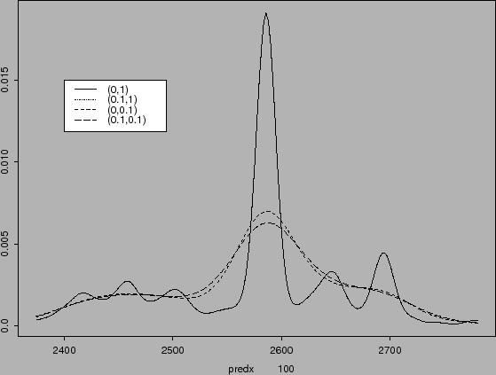
In Figure 2 the effect of changing the prior is observable:
On initially examining Figure 2, it is apparent that 1 and 2 show the same curve, the weak prior is overridden by the data. In 3 and 4 the curves are similar and smooth, the information in the data being insufficient to override the strong prior.
Having a degree of belief in the confidence placed in an ``expert opinion''
is central to a subjective Bayesian approach to a problem. Priors arising from
either previous knowledge of a process or from some reliable analysis of a
situation may be assumed to have some degree of validity. This is
expressed here in 3 and 4 by the adoption of a small value
for ![]() leading to the retention of the smooth curve in the density
estimate. The larger prior value for
leading to the retention of the smooth curve in the density
estimate. The larger prior value for ![]() in 1 and 2
expresses the opposite, i.e. an assumption that there is no prior belief in a
smooth curve and that is reflected in the density estimation obtained. Equally
a strong belief in a jagged curve could be imposed, which would seem to be more
appropriate here. In all cases, more data reduces the influence of the prior.
in 1 and 2
expresses the opposite, i.e. an assumption that there is no prior belief in a
smooth curve and that is reflected in the density estimation obtained. Equally
a strong belief in a jagged curve could be imposed, which would seem to be more
appropriate here. In all cases, more data reduces the influence of the prior.
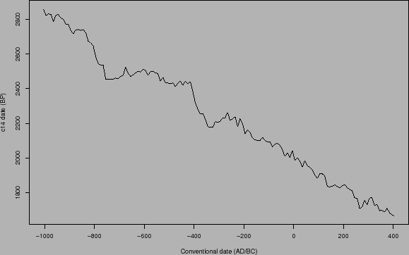
Finally, note that the jagged curve in 1 and 2 might be taken
to indicate that the curve is under smoothed, however, the ![]() calibration
curve used here is in nowise linear as can be seen in Figure 3, and
this might be reflected in the posterior.
calibration
curve used here is in nowise linear as can be seen in Figure 3, and
this might be reflected in the posterior.
danny 2009-07-23