Next: Marginal and conditional densities Up: The Bayesian paradigm Previous: The Bayesian paradigm
Consider a model for data
![]() assumed to be observed values
of some random variable
assumed to be observed values
of some random variable
![]() . This model defines a probability
distribution for
. This model defines a probability
distribution for
![]() in terms of parameters
in terms of parameters
![]() , from
a parameter space
, from
a parameter space
![]() , by a density
function
, by a density
function
![]() . The value of this density data
. The value of this density data
![]() is often
called the likelihood function as it describes the
likelihood of this particular sample
is often
called the likelihood function as it describes the
likelihood of this particular sample
![]() in terms of the parameters
in terms of the parameters
![]() .
.
In a Bayesian model initial knowledge
about
![]() is represented as a prior distribution having
density
is represented as a prior distribution having
density
![]() . This may come from some `expert'
assessment of the parameter value or from some previous measurement
or experiment. Statistical inference
for
. This may come from some `expert'
assessment of the parameter value or from some previous measurement
or experiment. Statistical inference
for
![]() is obtained by using Bayes' Theorem to update
knowledge about
is obtained by using Bayes' Theorem to update
knowledge about
![]() in the light of the sample data
in the light of the sample data
![]() .
.
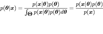
The inference about
![]() , given data
, given data
![]() , is provided
by the posterior density given by Bayes' Theorem as:
, is provided
by the posterior density given by Bayes' Theorem as:
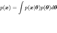
where
![]() is the entire parameter space.
is the entire parameter space.
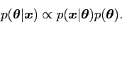
It is often convenient and sufficient to express Bayes' theorem to proportionality1 as
Note that
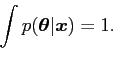
is obtainable as the constant needed to make
![]() a proper density, so that
a proper density, so that
 |
(4) |
If the sample is large then the information contained in the prior is swamped by that in the data and the prior has little effect on the posterior density. If, on the other hand, the sample information is small the posterior will be dominated by the prior.
The Bayesian approach has several theoretical advantages over, for
example, the more familiar frequentist methods. One such is that it
does not violate the
likelihood principle which implies that all the information to be
learned about
![]() from the sample is captured in the
likelihood (Lindley, 1965). Hence, two different samples having proportional
likelihoods would have the same inference; this is true if Bayesian
methods are used, see, for example, Savage (1962) and
O'Hagan (1994). As a simple example of a statistic in common use
that violates the likelihood principle consider the problem of
estimating variance (
from the sample is captured in the
likelihood (Lindley, 1965). Hence, two different samples having proportional
likelihoods would have the same inference; this is true if Bayesian
methods are used, see, for example, Savage (1962) and
O'Hagan (1994). As a simple example of a statistic in common use
that violates the likelihood principle consider the problem of
estimating variance (![]() )
)
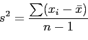 |
(5) |
where
![]() sample mean and
sample mean and ![]() sample size,
sample size, ![]() is an unbiased
estimator for
is an unbiased
estimator for ![]() . The denominator has been chosen to remove
bias thus considering samples that have not been seen and, hence,
information not in the observed data.
. The denominator has been chosen to remove
bias thus considering samples that have not been seen and, hence,
information not in the observed data.