Next: Discussion Up: A Bayesian Kernel Density Previous: Sawtooth Density
Outputs from the Grand Tour can be projections onto subspaces of any
dimensionality, usually one two or three for convenience, as discussed in
section ![]() . Extending the BKDE discussed above
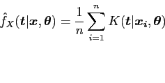
to more than one dimension is both natural and easy. A KDE is still specified in
terms of some function
. Extending the BKDE discussed above
to more than one dimension is both natural and easy. A KDE is still specified in
terms of some function
![]() and an estimate of
and an estimate of
![]() based on the sample
based on the sample
![]() , at the point,
, at the point,
![]() is written
as
is written
as
 |
(27) |
where
 |
(28) |
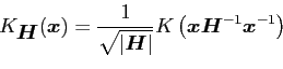
![]() is a bandwidth matrix and
is a bandwidth matrix and ![]() is some bivariate kernel.
is some bivariate kernel.
The estimate of ![]() based on the sample
based on the sample
![]() , at the
point
, at the
point
![]() ,
,
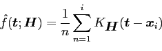
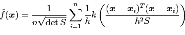
![]() is seen to again be of the form
is seen to again be of the form
where ![]() is the number of data items. Note that
is the number of data items. Note that
![]() may be considered
to be a generalisation of bandwidth. Taking
may be considered
to be a generalisation of bandwidth. Taking
![]() with univariate
data still leads to the standard KDE of (1), however, taking
with univariate
data still leads to the standard KDE of (1), however, taking
![]() leads to some higher dimensional estimate. In this case interest
is in bivariate data and a
leads to some higher dimensional estimate. In this case interest
is in bivariate data and a ![]() matrix form of
matrix form of
![]() .
.
There are three possible orders of complexity for
![]() ; if
; if
![]() , the class of all symmetric, positive, definite
, the class of all symmetric, positive, definite
![]() matrices, then there are 3 bandwidth parameters to
choose; if
matrices, then there are 3 bandwidth parameters to
choose; if ![]() , the subclass of all diagonal, positive,
definite
, the subclass of all diagonal, positive,
definite ![]() matrices, then there are 2 bandwidth parameters
to choose; and finally, if
matrices, then there are 2 bandwidth parameters
to choose; and finally, if ![]() , where
, where
![]() , there is only 1 bandwidth parameter to choose.
, there is only 1 bandwidth parameter to choose.
However, a compromise between the work needed to estimate the bandwidth and the
time taken to perform the estimation is required. Fukunaga (1972, p. 175)
suggests a simple way of obtaining a bandwidth matrix of arbitrary orientation
(see Silverman, 1986, p. 78). Take
![]() to be of the form
to be of the form
| (30) |
where
![]() is the covariance matrix. This approach is equivalent
to sphering the data (i.e. transforming it to have unit
covariance matrix).
is the covariance matrix. This approach is equivalent
to sphering the data (i.e. transforming it to have unit
covariance matrix).
This gives an estimate of the form
 |
(31) |
It can be shown (Wand and Jones, 1995, p. 106) that, for the
multivariate
![]() distribution, the Asymptotic Mean
Integrated Squared Error (AMISE) optimal
distribution, the Asymptotic Mean
Integrated Squared Error (AMISE) optimal
![]() satisfies
satisfies
| (32) |
for a scalar constant ![]() . This implies that, for the multivariate Normal,
sphering is appropriate. There is, unfortunately, no equivalent result for
estimation of arbitrary density shapes. This is the approach taken for the
version of the bivariate BKDE incorporated into the Grand Tour. By taking
. This implies that, for the multivariate Normal,
sphering is appropriate. There is, unfortunately, no equivalent result for
estimation of arbitrary density shapes. This is the approach taken for the
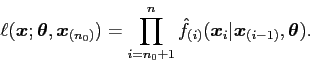
version of the bivariate BKDE incorporated into the Grand Tour. By taking ![]() to be a
model for the data a likelihood function is constructed as before.
to be a
model for the data a likelihood function is constructed as before.
 |
(33) |
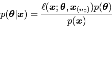
Choice of prior for
![]() again indicates belief in the
smoothness of the underlying density and in the strength of that
belief. This gives the posterior density
again indicates belief in the
smoothness of the underlying density and in the strength of that
belief. This gives the posterior density
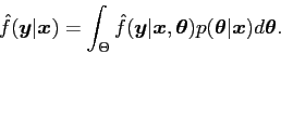
and the predictive density
danny 2009-07-23