Next: Numerical approach Up: Implementation Example Previous: Simulation approach
As above the likelihood is
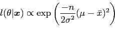 |
(34) |
so the log-likelihood is
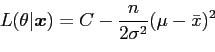 |
(35) |
where ![]() is a constant. Differentiating and equating to zero gives
is a constant. Differentiating and equating to zero gives
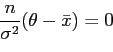 |
(36) |
so that
| (37) |
and a second differentiation gives
 |
(38) |
giving, in this case, ![]() and
and
![]() .
.
A histogram of 1000 samples from
![]() is shown in
figure 3. While not a good density estimator, a histogram is useful
for the gross comparison of two samples needed here. Note that this histogram
appears to come from a distribution with a smaller standard deviation than that
shown in figure 1; the predictive sample is a safer estimate as it
allows for the uncertainty in the point density estimation.
is shown in
figure 3. While not a good density estimator, a histogram is useful
for the gross comparison of two samples needed here. Note that this histogram
appears to come from a distribution with a smaller standard deviation than that
shown in figure 1; the predictive sample is a safer estimate as it
allows for the uncertainty in the point density estimation.
danny 2009-07-23